
When XGBoost Shines
And when it doesn't.

Let’s take a break from Neural Networks and Transformers for a moment, because not every Machine Learning (ML) problem needs convolutional or attention layers. This is especially true when working with structured data such as tabular data in a CSV file (rather than image or text), which often does not benefit from deep architectures.
This is where XGBoost still shines. Depending on your background, you might wonder: What makes XGBoost so special? Unsurprisingly, eXtreme Gradient Boosting (XGBoost) is a boosted tree algorithm with some useful upgrades. In the words of its creator, “XGBoost scales to billions of examples and uses very few resources.”1 It scales well with billions of samples in the dataset, and it’s fast. What’s more, it even handles missing data (I’ll leave the specifics to my curious readers). Next to these features, a regularization term is added to its objective function to help control overfitting, something standard gradient boosting didn’t originally account for.
So, is it the winning algorithm that hits state-of-the-art (SOTA) performance on every dataset, every time? XGBoost gained popularity for a reason, especially among Kaggle competitors. In many real-world cases, it exhibits impressive performance.
To understand how XGBoost builds on earlier methods, it helps to revisit tree-based algorithms briefly. It starts with Decision Trees, which are simple and interpretable models that split data based on rules. Then come Random Forests, which train many trees independently and combine their outputs, using averaging for regression or majority voting for classification. This is called bagging, and it helps reduce variance.
Boosting takes a different approach. Instead of training trees in parallel, it builds them sequentially. Each new tree focuses on correcting the errors made by the previous ones2. This process turns a group of weak learners into a strong model. Among boosting methods, Gradient Boosting became especially popular by framing this correction process as an optimization problem.
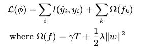
XGBoost builds on this foundation with improvements like regularization (see the second term (Ω) of the objective function in Figure 1). Its objective function does more than just minimize the loss. It also penalizes the complexity of the model, which helps to avoid overfitting3.
Under the hood, XGBoost uses gradient descent4 to optimize each new tree it adds to the ensemble. At each iteration, it adjusts parameters to minimize a cost function. While this resembles standard gradient boosting, XGBoost adds refinements that speed up training and improve generalization.
All of this makes XGBoost a powerful algorithm, but also a sensitive one. In my experience, small changes in hyperparameters5 can lead to noticeably different results. [🔔 Click here in case you need to refresh your knowledge on hyperparameter tuning.] Before we go into the most important tunable parameters, let me highlight the importance of setting a fixed random seed. This ensures your results are reproducible. Some of the most impactful parameters include:
max_depth: controls the maximum depth of each tree. Increasing this value will make the model more complex and more likely to overfit.
learning_rate: determines the step size at each boosting step to prevent overfitting.
scale_pos_weight: controls the balance of positive and negative weights, so very useful for handling imbalanced datasets.
reg_alpha and reg_lambda: control L1 and L2 regularization terms on weights, respectively.
colsample_bytree: specifies the fraction of features to consider when building each tree.

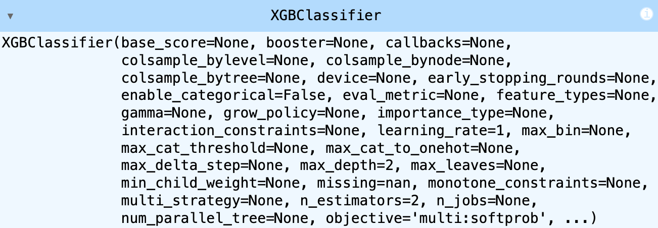
Figure 2: List of parameters from XGBClassifier
Like most ML algorithms, XGBoost also struggles with heavily imbalanced data. When the minority class is very small, simple oversampling or undersampling6 might not help. But including the scale_pos_weight as a hyperparameter can improve learning in these cases. It's not a perfect fix, but it's a useful lever.
Each of these parameters (and many others, some of which are shown in Figure 2) can significantly impact model performance. However, achieving SOTA performance results on training and test data with ML models takes more than just calling a fit() function from a library like sklearn or xgboost. If you use such libraries, it is easy to train an XGBoost model. That’s why I feel like training XGBoost is a leaky abstraction to some extent. These libraries often assign default parameter values, which most probably do not align well with your specific data or use case. To build reliable models, we need thoughtful data preprocessing7, effective feature engineering, careful hyperparameter tuning, thorough evaluation, and attention to deployment. Even seemingly small choices, like how to encode categorical features, can affect performance.

Hyperparameter tuning can become overwhelming, especially with XGBoost’s extensive search space of possible hyperparameter values, as shown in Figure 2. A full Grid search (see GridSearchCV from sklearn) tries every combination of specified values. Although trying out every possible combination with grid search seems like the most thorough strategy, this method can quickly become too slow and resource-intensive. A more efficient option is Random search (see RandomizedSearchCV from sklearn), which selects hyperparameter combinations at random and can yield comparable results with significantly fewer evaluations. Each combination you try requires training the model and evaluating it on validation data, so reducing the total number of these evaluations can save a lot of time and computation. As an alternative, Bayesian optimization optimizes objective functions that take a long time (minutes or hours) to evaluate. It builds a surrogate for the objective and quantifies the uncertainty in that surrogate using a Bayesian ML technique, Gaussian process regression, and then uses an acquisition function defined from this surrogate to decide where to sample (the next set of parameters)8.
Once you find the best hyperparameters, computation time becomes increasingly important, especially as you move toward production. More importantly, for yourself, stakeholders, and end users, how and why an ML model arrived at its prediction are as important as the prediction. Regulations like the EU AI Act further emphasize users’ right to explanation. This is where early stopping becomes especially useful.
xgboost_model.fit(X_train, y_train, early_stopping_rounds=30, …)Instead of running hundreds of boosting rounds just because you can (with n_estimators as the controlling hyperparameter), early stopping allows you to monitor validation performance and halt training when improvements start to level off9. In my experience, this saves time and produces a smaller, more explainable model.
In the end, XGBoost is indeed a strong and advanced ML algorithm. It handles large datasets, captures non-linear relationships, and can work reasonably well with imbalanced data to some extent. But no algorithm works in every case. What matters most is understanding how it works, when to use it, and what its limitations are. You're now ready to explore XGBoost further and start building your own models using the xgboost and sklearn Python libraries.
https://web.archive.org/web/20160807033610/http://homes.cs.washington.edu/~tqchen/2016/03/10/story-and-lessons-behind-the-evolution-of-xgboost.html
Bagging and boosting are examples of ensemble learning, where multiple models are combined to improve predictive performance.
Chen, Tianqi, and Carlos Guestrin. “XGBoost: A scalable tree boosting system.” Proceedings of the 22nd acm sigkdd international conference on knowledge discovery and data mining. 2016.
https://www.3blue1brown.com/lessons/gradient-descent
https://xgboost.readthedocs.io/en/stable/parameter.html
https://en.wikipedia.org/wiki/Oversampling_and_undersampling_in_data_analysis
Depending on your data and the ML model you plan to use, data preprocessing may include normalization, bucketing, imputation, and encoding of categorical features.
Frazier, Peter I. “A tutorial on Bayesian optimization.” arXiv preprint arXiv:1807.02811. 2018.
This works well for XGBoost, where validation performance tends to be stable. With Neural Networks, however, stopping the model training when the validation loss seems to be leveling off requires more attention.